Comparing Modern Scalable Hyperparameter Tuning Methods

In this post, we’ll compare the following hyper-parameter optimization methods.

Random Search
Bayesian Search using HyperOpt
Bayesian Search combined with Asynchronous Hyperband
Population-Based Training

Experiment

we’ll train a simple DCGAN on the MNIST dataset and optimize the model for maximizing the inception score.

We’ll use Ray Tune to perform these experiments and track the results on the W&B dashboard.

I also did a video on my channel that goes in-depth in explaining this experiment -

Link to the Live Dashboard

The Search Space

We’ll use the same search space for all the experiments in order to make the comparison fair.

config = {
        "netG_lr": lambda: np.random.uniform(1e-2, 1e-5),
        "netD_lr": lambda: np.random.uniform(1e-2, 1e-5),
        "beta1": [0.3,0.5,0.8]
}

Let’s perform a random search across the search space to see how well it optimizes. This will also act as the baseline metric for our comparison. Our experimental setup has 2 GPUs and 4 CPUs. We’ll parallelize the operation across multiple GPUs. Ray Tune does this automatically for you if you specify the resources_per_trail.

analysis = tune.run(
    dcgan_train,
    resources_per_trial={'gpu': 1,'cpu':2}, # Tune will use this information to parallelize the tuning operation
    num_samples=10,
    config=config
)

Let’s see the results

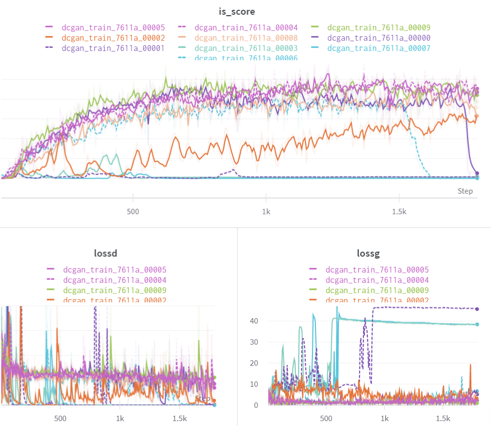
Weights & Biases panels for the random search: inception score against training step for ten DCGAN runs, most plateauing between 4 and 6 while two collapse to zero, plus discriminator and generator loss panels below. — Image by author

Inference: random search

As expected, we get varied results.

Some of the models did optimize as the tuner got lucky and chose the right set of hyper-parameters
but some models’ inception score graph remained flat as they did not optimize due to bad hyper-parameter values.
Thus, when using a random search, you might end up reaching the optimal value but you definitely end up wasting a lot of resources on the runs that don’t add any value.

The basic idea behind Bayesian Hyperparameter tuning is to not be completely random in your choice for hyper-parameters but instead use the information from the prior runs to choose the hyperparameters for the next run. Tune supports HyperOpt which implements Bayesian search algorithms. Here’s how you do it.

Here’s what results look like

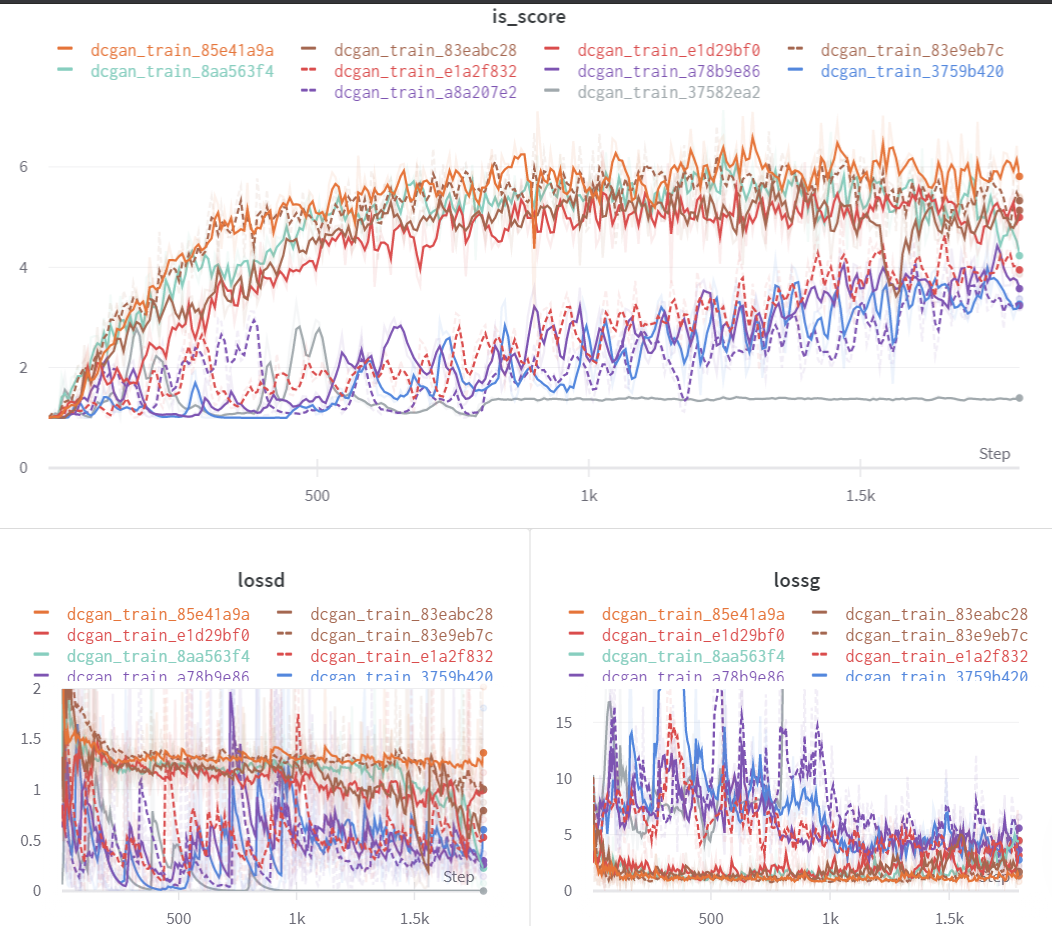
Weights & Biases inception-score and loss panels for the Bayesian (HyperOpt) search runs, plotted against training step. — Image by author

Inference: Bayesian search

There are significant improvements compared to the previous run as there is only 1 flat curve.
This implies that the search algorithm chose the hyper-parameter values based on the results of previous runs.
On average, the runs performed better than random search
Resource wastage can be avoided by terminating the bad runs earlier.

The idea Asynchronous Hyperband is to eliminate or terminate the runs that don’t perform well. It makes sense to combine this method with the Bayesian search to see if we can further reduce the wastage of resources on the runs that don’t optimize. We just need to make a small change in our code to accommodate Hyperband.

Let us now see how this performs

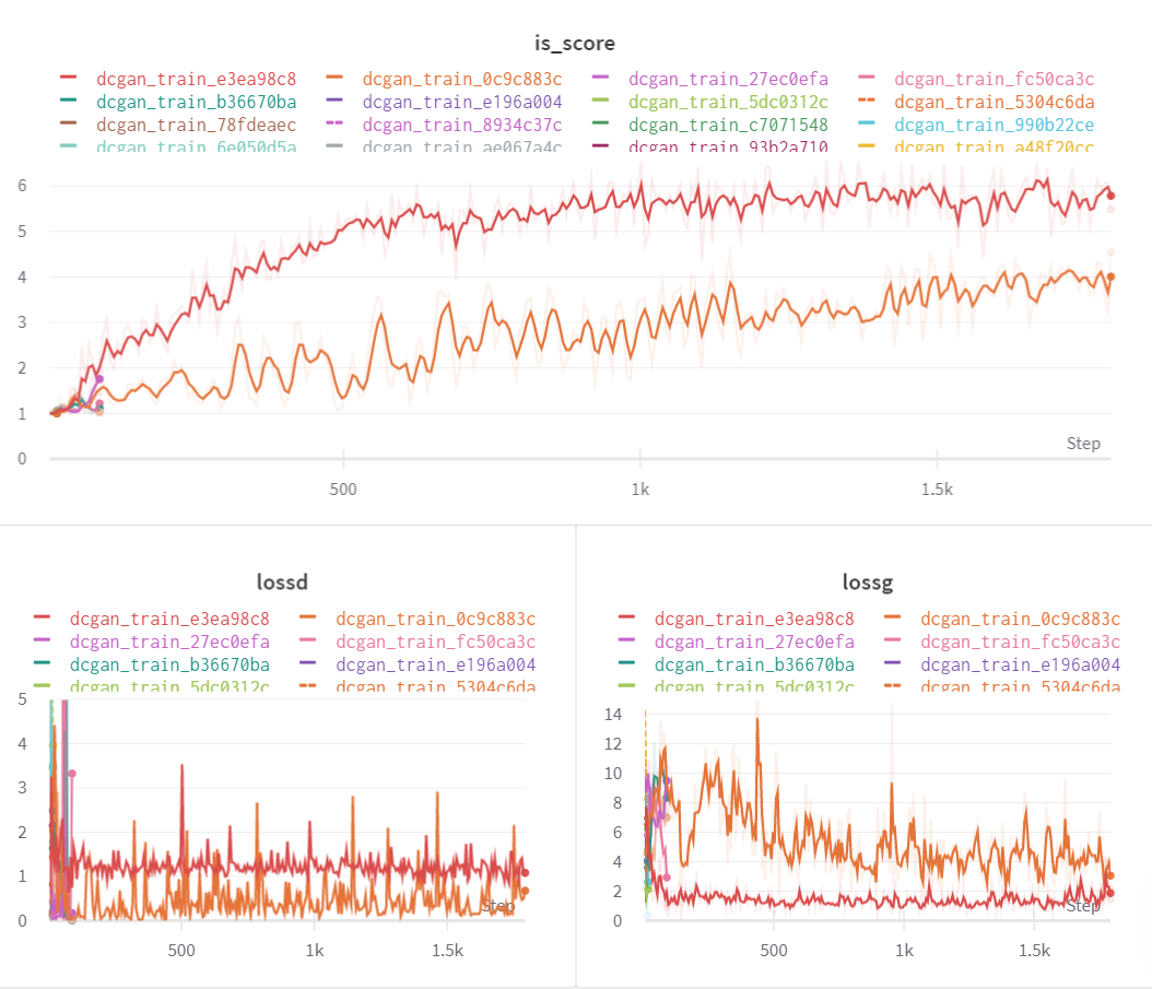
Weights & Biases panels for Bayesian search with Hyperband: most of the twelve runs stop within the first hundred steps, leaving two that continue, one reaching about 5.8 inception score and the other about 4, with the loss panels below. — Image by author

Inference: Bayesian search with Hyperband

Only 2 out of 20 runs were executed for defined epochs while others were terminated earlier.
The highest accuracy achieved was still slightly higher than the runs without the Hyperband scheduler.
Thus, by terminating bad runs early on in the training process, we have not only speeded up the tuning job but also saved compute resources.

Population-Based Training illustration — Image source: the companion W&B report

The last tuning algorithm that we’ll cover is population-based training (PBT) introduced by Deepmind research. The basic idea behind the algorithm in layman terms:

Run the optimization process for some samples for a given time step(or iterations) T.
After every T iterations, compare the runs and copy the weights of good performing runs to the bad performing runs and change their hyper-parameter values to be close to the values of the runs that performed well.
Terminate the worst-performing runs. Although the idea behind the algorithm seems simple, there is a lot of complex optimization math that goes into building this from scratch. Tune provides a scalable and easy-to-use implementation of the SOTA PBT algorithm

Let us now look at the results.

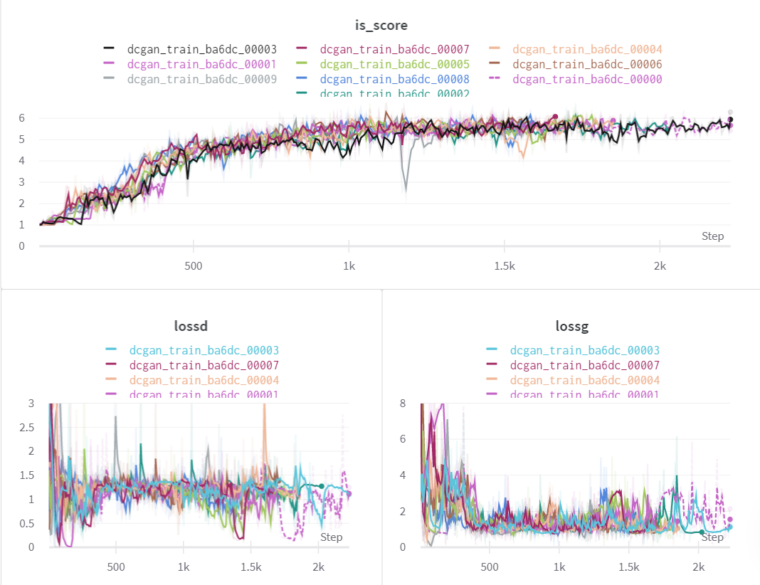
Weights & Biases inception-score and loss panels for the population-based training runs, plotted against training step. — Image by author

Inference: population-based training

The results look quite surprising. There are multiple factors that are unique about these results.

Almost all the runs have reached the optimal point
The highest score( of 6.29) was achieved by one of the runs
The runs that started off as bad performers or outliers have also converged as the experiment proceeded.
There are no runs that have a flat inception score graph
Some bad performing runs were stopped in the middle of the process
Thus, no resource has been wasted on bad runs

The answer is the hyper-parameter mutation done by the PBT scheduler. After every T time steps, the algorithm also mutates the values of hyper-parameters to maximize the desired metric. Here's how the parameters were mutated by the PBT scheduler for this experiment.

Let us now see how the hyper-parameters were adjusted by the PBT algorithm to maximize the inception score

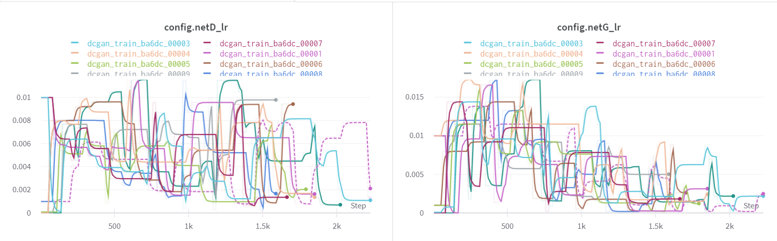
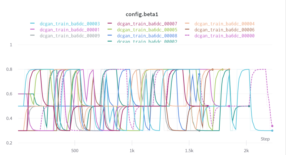
Two panels showing the discriminator and generator learning rates being mutated by the population-based training scheduler: each run's rate steps up and down in flat segments over training rather than following a fixed schedule, and all runs trend downward after roughly step 1000. — Image by author

Continuation of the population-based training parameter mutation charts, showing how the scheduler adjusted hyperparameters to maximise the inception score. — Image by author

The hyper-parameter values are constantly adjusted throughout the experiment.
The runs that start off with a bad hyper-parameter value are soon updated.
PBT operates on explore and exploit methodology exploring the space for good parameter values and exploits by updating the bad runs.

We’ll now reduce the number of runs to 5 in order to make things difficult for PBT. Let’s see how it performs under this restricted circumstance.

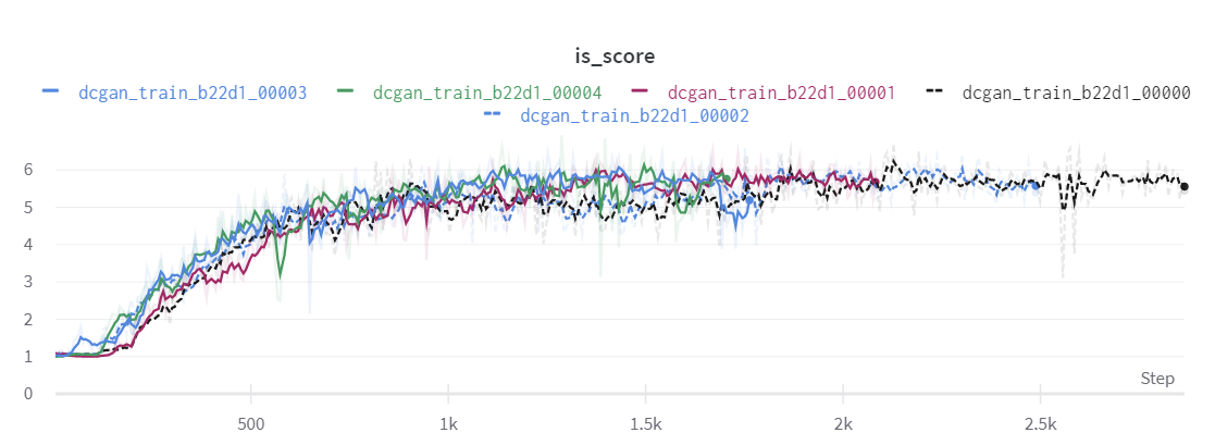
Inception score against step for population-based training restricted to five runs: all five climb together to roughly 5.5 to 6 by step 1000 and hold there, with no run left behind. — Image by author

Even after reducing the number of runs to 5, PBT optimizer still outperforms random search and bayesian optimization.
As expected, the bad performing runs were terminated early on in the training process

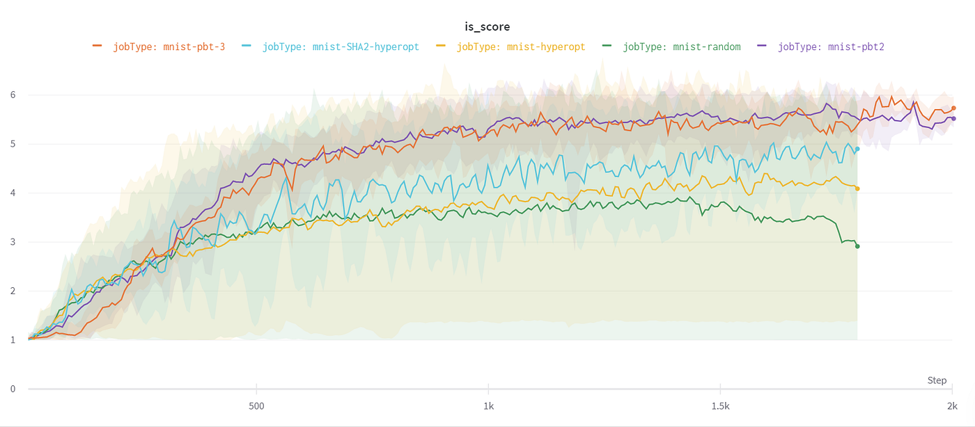
Here’s how the final comparison of the average inception scores looks like. We’ve averaged across 5 run sets:

Random Search — 10 Runs ( Job Type — mnist-random)
Bayesian Search — 10 Runs ( Job Type — mnist-hyperopt)
Bayesian Search with Hyperband — 20 Runs (Job Type- mnist-SHA2-hyperopt)
PBT scheduler — 10 Runs (Job Type — mnist-pbt2)
PBT scheduler — 5 Runs (Job Type — mnist-pbt3)

Inception score against step averaged across the five job types: both population-based training runs reach about 5.5 to 5.8, Bayesian search with Hyperband about 4.9, plain Bayesian search about 4.1, and random search about 2.9. — Image by author

If you enjoyed reading this, you can follow me on twitter to get more updates. I also make deep learning videos on my youtube channel.